A more efficient loss function for Siamese
At work, we are working with Siamese Neural Net (NN) for one shot training on telecom data. Our goal is to create a NN that can easily detect failure in Telecom Operators networks. To do so, we are building this N dimension encoding to describe the actual status of the network. With this encoding we can then evaluate what is the status of network and detect faults. This encoding as the same goal as something like word encoding (Word2Vec or others). To train this encoding we use a Siamese Network [Koch et al.] to create a one shot encoding so it would work on any network. A simplified description of Siamese network is available here. For more details about our experiment you can read the blog of my colleague who is the master brain behind this idea.
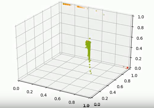
The current experiment, up to now is working great. This network can split the different traffic scenarios. As you can see on this picture, the good traffic (Green) is easily spitted away from error type 1 (Red) and error type 2 (Orange)
THE PROBLEM
So what is the problem, it seems to work fine, doesn’t it? After some reflection I realized that there was a big flaw in the loss function.
First here is the code for our model. (Don’t have to read all the code, I will point out the issue.
def triplet_loss(y_true, y_pred, alpha = 0.4):
    """
    Implementation of the triplet loss function
    Arguments:
    y_true -- true labels, required when you define a loss in Keras, you don't need it in this function.
    y_pred -- python list containing three objects:
            anchor -- the encodings for the anchor data
            positive -- the encodings for the positive data (similar to anchor)
            negative -- the encodings for the negative data (different from anchor)
    Returns:
    loss -- real number, value of the loss
    """

    anchor = y_pred[:,0:3]
    positive = y_pred[:,3:6]
    negative = y_pred[:,6:9]

    # distance between the anchor and the positive
    pos_dist = K.sum(K.square(anchor-positive),axis=1)

    # distance between the anchor and the negative
    neg_dist = K.sum(K.square(anchor-negative),axis=1)

    # compute loss
    basic_loss = pos_dist-neg_dist+alpha
    loss = K.maximum(basic_loss,0.0)

    return loss

def create_base_network(in_dims, out_dims):
    """
    Base network to be shared.
    """
    model = Sequential()
    model.add(BatchNormalization(input_shape=in_dims))
    model.add(LSTM(512, return_sequences=True, dropout=0.2, recurrent_dropout=0.2, implementation=2))
    model.add(LSTM(512, return_sequences=False, dropout=0.2, recurrent_dropout=0.2, implementation=2))
    model.add(BatchNormalization())
    model.add(Dense(512, activation='relu'))
    model.add(BatchNormalization())
    model.add(Dense(out_dims, activation='linear'))
    model.add(BatchNormalization())

    return model

in_dims = (N_MINS, n_feat)
out_dims = N_FACTORS

# Network definition
with tf.device(tf_device):

    # Create the 3 inputs
    anchor_in = Input(shape=in_dims)
    pos_in = Input(shape=in_dims)
    neg_in = Input(shape=in_dims)

    # Share base network with the 3 inputs
    base_network = create_base_network(in_dims, out_dims)
    anchor_out = base_network(anchor_in)
    pos_out = base_network(pos_in)
    neg_out = base_network(neg_in)
    merged_vector = concatenate([anchor_out, pos_out, neg_out], axis=-1)

    # Define the trainable model
    model = Model(inputs=[anchor_in, pos_in, neg_in], outputs=merged_vector)
    model.compile(optimizer=Adam(),
                  loss=triplet_loss)

# Training the model
model.fit(train_data, y_dummie, batch_size=256, epochs=10)
My issue is with this line of the loss function.
‘loss = K.maximum(basic_loss,0.0)’
There is a major issue here, every time your loss gets below 0, you loose information, a ton of information. First let’s look at this function.
It basically does this:
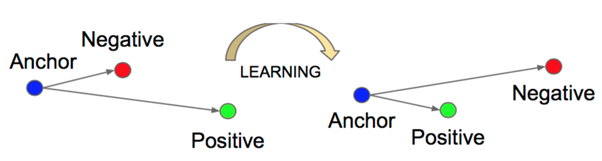
It tries to bring close the Anchor (current record) with the Positive (A record that is in theory similar with the Anchor) as far as possible from the Negative (A record that is different from the Anchor).
The actual formula for this loss is:

This process is detailed in the paper FaceNet: A Unified Embedding for Face Recognition and Clustering by Florian Schroff, Dmitry Kalenichenko and James Philbin.
So as long as the negative value is further than the positive value + alpha there will be no gain for the algorithm to condense the positive and the anchor. Here is what I mean:
Let’s pretend that:
- Alpha is 0.2
- Negative Distance is 2.4
- Positive Distance is 1.2
The loss function result will be 1.2–2.4+0.2 = -1. Then when we look at Max(-1,0) we end up with 0 as a loss. The Positive Distance could be anywhere above 1 and the loss would be the same. With this reality, it’s going to be very hard for the algorithm to reduce the distance between the Anchor and the Positive value.
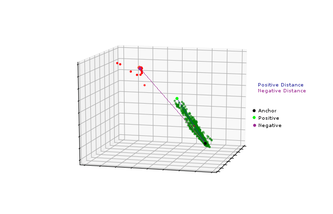
As a more visual example, here is 2 scenarios A and B. They both represent what the loss function measure for us.
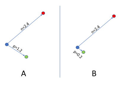
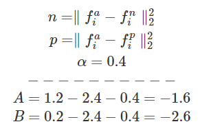
After the Max function both A and B now return 0 as their loss, which is a clear lost of information. By looking simply, we can say that B is better than A.
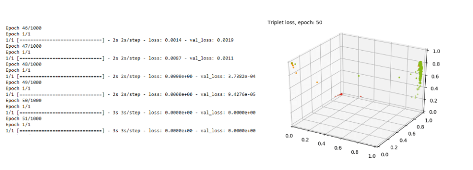
In other words, you cannot trust the loss function result, as an example here is the result around Epoch 50. The loss (train and dev) is 0, but clearly the result is not perfect.
OTHER LOSSES
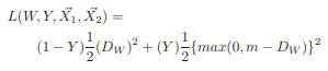
Another famous loss function the contrastive loss describe by Yan LeCun and his team in their paper Dimensionality Reduction by Learning an Invariant Mapping is also maxing the negative result, which creates the same issue.
With the title, you can easily guess what is my plan… To make a loss function that will capture the “lost” information below 0. After some basic geometry, I realized that if you contain the N dimension space where the loss is calculated you can more efficiently control this. So the first step was to modify the model. The last layer (Embedding layer) needed to be controlled in size. By using a Sigmoïde activation function instead of a linear we can guarantee that each dimension will be between 0 and 1.

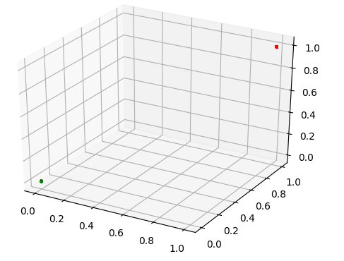
Then we could assume that the max value of a distance would be N. N being the number of dimensions. Example, if my anchor is at 0,0,0 and my negative point is at 1,1,1. The distance based on Schroff formula would be 1²+1²+1² = 3. So if we take into account the number of dimensions, we can deduce the max distance. So here is my proposed formula.
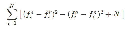
Where N is the number of dimensions of the embedding vector. This look very similar, but by having a Sigmoïde and a proper setting for N, we can guarantee that the value will stay above 0.
FIRST RESULTS
After some initial test, we ended up with this model.
 On the good side we can see that all the points from the same cluster get super tight, even to the point that they become the same. But on the downside it turns out that the two error cases (Orange and Red) got superimposed.
The reason for this is the loss is smaller like this then when the Red and Orange split. So we needed to find a way to break the cost linearity; In other words, make it really costly as more the error grows.
Non-Linearity
Instead of the linear cost we proposed a non-linear cost function:

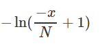 Where the curve is represented by this ln function when N = 3
With this new non-linearity, our cost function now looks like:
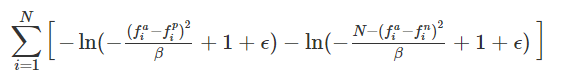 Where N is the number of dimensions (Number of output of your network; Number of features for your embedding) and β is a scaling factor. We suggest setting this to N, but other values could be used to modify the non-linearity cost.
As you can see, the result speaks for itself:
 We now have very condensed cluster of points, way more than the standard triplet function result.
As a reference here is the code for the loss function.
def lossless_triplet_loss(y_true, y_pred, N = 3, beta=N, epsilon=1e-8):
    """
    Implementation of the triplet loss function

    Arguments:
    y_true -- true labels, required when you define a loss in Keras, you don't need it in this function.
    y_pred -- python list containing three objects:
            anchor -- the encodings for the anchor data
            positive -- the encodings for the positive data (similar to anchor)
            negative -- the encodings for the negative data (different from anchor)
    N  --  The number of dimension
    beta -- The scaling factor, N is recommended
    epsilon -- The Epsilon value to prevent ln(0)

    Returns:
    loss -- real number, value of the loss
    """
    anchor = tf.convert_to_tensor(y_pred[:,0:N])
    positive = tf.convert_to_tensor(y_pred[:,N:N*2])
    negative = tf.convert_to_tensor(y_pred[:,N*2:N*3])

    # distance between the anchor and the positive
    pos_dist = tf.reduce_sum(tf.square(tf.subtract(anchor,positive)),1)
    # distance between the anchor and the negative
    neg_dist = tf.reduce_sum(tf.square(tf.subtract(anchor,negative)),1)

    #Non Linear Values

    # -ln(-x/N+1)
    pos_dist = -tf.log(-tf.divide((pos_dist),beta)+1+epsilon)
    neg_dist = -tf.log(-tf.divide((N-neg_dist),beta)+1+epsilon)

    # compute loss
    loss = neg_dist + pos_dist

    return loss
Keep in mind, for it to work you need your NN last layer to be using a Sigmoïde activation function.

Even after 1000 Epoch, the Lossless Triplet Loss does not generate a 0 loss like the standard Triplet Loss.
DIFFERENCES
Based on the cool animation of his model done by my colleague, I have decided to do the same but with a live comparison of the two losses function. Here is the live result were you can see the standard Triplet Loss (from Schroff paper) on the left and the Lossless Triplet Loss on the right:
CONCLUSION
This loss function seems good, now I will need to test it on more data, different use cases to see if it is really a robust loss function. Let me know what you think about this loss function.
REFERENCES
- Koch, Gregory, Richard Zemel, and Ruslan Salakhutdinov. “Siamese neural networks for one-shot image recognition.” ICML Deep Learning Workshop. Vol. 2. 2015.
- Mikolov, Tomas, et al. “Efficient estimation of word representations in vector space.” arXiv preprint arXiv:1301.3781 (2013).
- Schroff, Florian, Dmitry Kalenichenko, and James Philbin. “Facenet: A unified embedding for face recognition and clustering.” Proceedings of the IEEE conference on computer vision and pattern recognition. 2015.
- Hadsell, Raia, Sumit Chopra, and Yann LeCun. “Dimensionality reduction by learning an invariant mapping.” Computer vision and pattern recognition, 2006 IEEE computer society conference on. Vol. 2. IEEE, 2006.
- https://thelonenutblog.wordpress.com/
- https://hackernoon.com/one-shot-learning-with-siamese-networks-in-pytorch-8ddaab10340e